spotify-analysis-medley / Medley of Music Analysis

Project description: Using a Spotify data set for all tracks from 1900 - 2021, I wanted to better understand what songs were most popular and which artists were most prolific. I also wanted to look closely to learn about the features or characteristics of the songs and how those categories might be related. I was able to observe there are many unique characterstics that make up a song, and may have more uniqueness than can be classified using features alone. I would like to continue to research this dataset further.

1. Data Cleaning and Analysis

First thing needed was to look at the data set as a whole and look at the data types and check for nulls.

track_df = pd.read_csv("....SpotifyDatasets//tracks.csv")
track_df.shape
track_df.info()
track_df.isnull().sum()

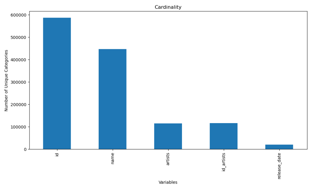
The datset has 20 columns, 586672 rows of data, and had 71 data fields that were null within the Name column. Once we removed the nulls, we can then check out the cardinality in columns that are object types. To visualize the Cardinality, I created bar graph to show the number of unique categories in the following: Id, Name, Artists, Artist_id, and Release Date.

#categories
track_cat = track_df.select_dtypes(include = 'object')
track_cat.info()
#cardinality
for col in track_cat.columns:
    print(f'{col}: {track_cat[col].nunique()}')
    print('/n')
#plot cardinality
track_cat.nunique().plot.bar(figsize=(12,6))
plt.ylabel('Number of Unique Categories')
plt.xlabel('Variables')
plt.title('Cardinality')

2. Which artists have the most songs on Spotify and which are most popular?

To look at which artists have the most songs on Spotify, we can do a simple count of songs by artist. I included a barplot to get a better visual. I learned that Die Drei is a popular German audio book series. I believe there are newer Spotify data sets that differentiate audio book/podcasts from songs. I had attempted to categorize songs by level of speechiness but found I could not easily distinguish podcasts from rap songs or other wordy song genres. This will be something I plan on coming back to.

#find artists with most songs
prolific_artists = track_df['artists'].value_counts().head(20)
prolific_artists

#barplot artists by sum of songs
fig, ax = plt.subplots(figsize = (12,10))
ax = sns.barplot(x = prolific_artists.values, y = prolific_artists.index, palette = 'rocket_r', orient = 'h', edgecolor = 'black', ax = ax)
ax.set_xlabel('Sum of Songs', c = 'r', fontsize = 12, weight = 'bold')
ax.set_ylabel('Artists',c = 'r', fontsize = 12, weight = 'bold')
ax.set_title('20 Most Prolific Artists on Spotify', c= 'r', fontsize = 14, weight = 'bold')
plt.show()

Next, I focused on poplularity, sorting the dataset based on the popularity column. After seeing the top 20 popular songs, I wanted to look closer at the artists and which had the most popular songs. I then took an average of popularity ranking of song by artist.

track_df = track_df.sort_values('popularity', ascending = False)
#20 most popular songs
top20 = track_df.head(20)
top20
artist_df =(track_df.groupby(['artists'], as_index=False).mean().groupby('artists')['popularity'].mean().sort_values(ascending=False))
artist_df.head(20)

I found the results insightful, and quickly added a few artists to list of artists to look up and listen to later. I did recognize several of the artists and was surprised to find Bad Bunny and Rosalia in the top 3.

3. Feature Correlation

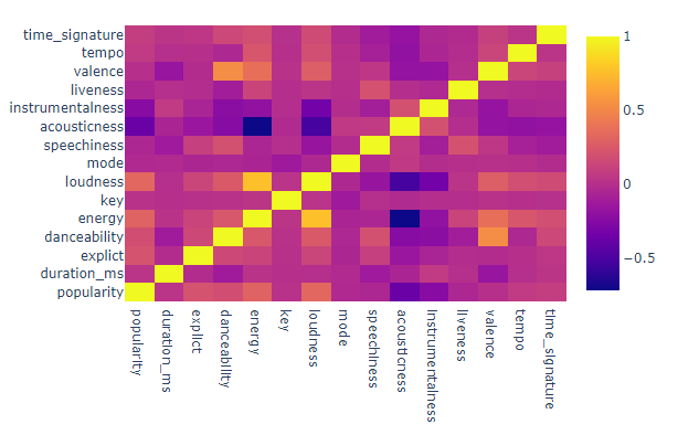
I wanted to see how the differernt song features were correlated. I created a heatmap to analyze the relationship between the characteristics. Looking at the map we can see that loudness and energy have to strongest correlation with a value of .765, and valence and danceability was next with a value of .528. Both of these correlated pairs make sense and was not shocked to see this translate to the graph.

#see correlation between any two given features with heatmap
import plotly.graph_objects as go
matrix = track_df.corr()
x_list=['popularity','duration_ms','explict','danceability','energy','key','loudness','mode','speechiness','acousticness','instrumentalness','liveness','valence','tempo','time_signature']
fig_heatmap = go.Figure(data=go.Heatmap(z=matrix,x=x_list,y=x_list,hoverongaps = False))
fig_heatmap.update_layout(margin=dict(t=200,r=200,b=200,l=200),width=800,height=650,autosize=False)
fig_heatmap.show()

4. Unsupervised Machine Learning with K-Means Clustering

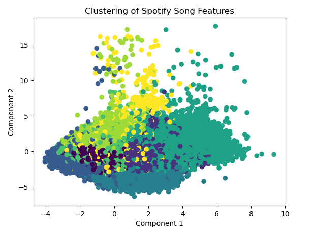
Without creating any training data we can use the K-Means algorithm to group the features by clusters and find the closest means. After calculating the z-score, we create a list to store the sum of squared distances for each cluster and then fit the model with the range of clusters. Using the Elbow Method, I decided to use 8 clusters. Using the silhouette score we can see the clusters are not going to be very prominent or far apart, with a silhoutee score of .15. As we continue to use a scatter plot, the clusters are found to be close together.

features = ['explicit','danceability','energy','key','loudness','mode','speechiness','acousticness','instrumentalness','liveness','valence','tempo','duration_ms']
df = track_df[features]
df = (df -df.mean()) / df.std()

#create an empty list to store sum of squared distances for each number of clusters
sse = []

#Fit the Kmeans model to the data with a range of different numbers of clusters
for k in range(1, 15):
        kmeans = KMeans(n_clusters=k)
        kmeans.fit(df)
#add the sum of squared distances for the current number of clusters to the list
        sse.append(kmeans.inertia_)
#plot the sum squared distances for each number of clusters for elbow method
plt.plot(range(1,15), sse)
plt.title('Elbow Method for Clustering')
plt.xlabel('Number of Clusters')
plt.ylabel('Sum of Squared Distances')
plt.show()
#Create the KMeans with 8 clusters
kmeans = KMeans(n_clusters=8, random_state=1)
#fit the data
kmeans.fit(df)
#Generate the clusters with KMeans via predict() model on the fitted KMeans model
clusters = kmeans.predict(df)

#print the cluster assignments for the first few data points
print(clusters[:10])
#Evaluate the quality of the generated clusters
silhouette_score(df, clusters)
# Visualize the clusters
#create two components
pca= PCA(n_components=2) 
#reduce to two dimensions using PCA
df_2d = pca.fit_transform(df)

#Plot the data points via scatter plot
plt.scatter(df_2d[:, 0],df_2d[:, 1], c=clusters)
plt.title('Clustering of Spotify Song Features')
plt.xlabel('Component 1')
plt.ylabel('Component 2')
plt.show()
#create two components
pca= PCA(n_components=2) 
#reduce to two dimensions using PCA
df_2d = pca.fit_transform(df)

#Plot the data points via scatter plot
plt.scatter(df_2d[:, 0],df_2d[:, 1], c=clusters)
plt.title('Clustering of Spotify Song Features')
plt.xlabel('Component 1')
plt.ylabel('Component 2')
plt.show()

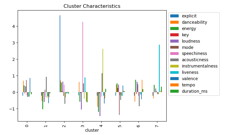
Next I assigned the clusters and flattened the array of subplots. Then grouped the features by means and created a bar plot to show the features by cluster.

#Unique cluster assignments
unique_clusters = np.unique(clusters)

#create grid of subplots
fig, axs = plt.subplots(nrows=4, ncols=2, figsize =(8, 8), sharex=True, sharey=True)

#flatten the array of subplots for easier iteration
axs = axs.flatten()

#iterate over the clusters
for i, cluster in enumerate(unique_clusters):
    #select the data points for current cluster
    df_cluster = df_2d[clusters == cluster]
    
    #Select the data points belonging to other clusters
    df_other_clusters = df_2d[clusters != cluster]
    
    #plot the data points belonging to other clusters in the grey
    axs[i].scatter(df_other_clusters[:,0], df_other_clusters[:,1], c='grey', label='Other Clusters', alpha =0.5)
    
    #plot the data points belonging to the current cluster with a different color
    axs[i].scatter(df_cluster[:, 0], df_cluster[:, 1], c='red', label='Cluster {}'.format(cluster))
    
    #set the x and y labels for the current subplot
    axs[i].set_xlabel('Component 1')
    axs[i].set_ylabel('Component 2')
    
    #add a legend to the current subplot
    axs[i].legend()
    
    plt.show()
clustered_df = df.copy()
clustered_df['cluster']= clusters

cluster_means = clustered_df.groupby('cluster').mean()
print(cluster_means)

cluster_means.plot(kind='bar')
plt.title('Cluster Characteristics')
plt.legend(bbox_to_anchor=(1.0, 1.0))
plt.show()

I noticed that explicit music can be associated with loudness and danceability and negatively associated with acousticness. Speechiness can somewhat be related with liveness and danceability and negatively associated with loudness. Instrumentalness can be associated with acousticness and negatively associated with loudness.

5. Further research and takeaways

I want to continue to try additional algorithms on this data and see what other insights I can find.